Fraud detection with TensorFlow and Explainable AI

Anomaly detection can be a good candidate for machine learning since it is often hard to write a series of rule-based statements to identify outliers in data. In this post I’ll look at building a model for fraud detection on financial data.

🚨If you’re thinking groan, that sounds boring, don’t go away just yet! Fraud detection addresses some interesting challenges in ML:

• Very imbalanced datasets: because anomalies are, well, anomalies, there are not many of them. ML works best when datasets are balanced, so things can get complicated when outliers make up less than 1% of your data.

• Need to explain results: if you’re looking for fraudulent activity, chances are you’ll want to know why a system flagged something as fraudulent rather than just take its word for it. Explainability tools can help with this.

Getting the data from Kaggle

Kaggle is my go-to place for finding all sorts of datasets and it did not disappoint here. Financial datasets specifically are hard to come by, so I ended up going with this synthetically generated one¹. While it is synthetic, it’s based on lots of ongoing research in this field. What’s included?

• 6.3 million rows, 8k of which are fraudulent transactions (a mere 0.1% of the whole dataset!)

• Each row includes data on the type of transaction ( transfer, payment, cash out, etc.), the amount in the originating account before and after the transaction, and the same for the receipient’s account

Accounting for imbalanced data

6.3M rows sounds great, right? In this case more data is not necessarily better. If I shove the data into a model as is, chances are the model will reach 99.9% accuracy by guessing every transaction is not a fraudulent one simply because 99.9% of the data is non fraudulent cases.

There are a few different approaches for dealing with imbalanced data, and I’m open to feedback on the approach I’m going with. To balance things out, I took all 8k of the fraudulent cases from the dataset along with a random sample of ~31k of the not fraud cases:

data = pd.read_csv('fraud_data.csv')

# Split into separate dataframes for fraud / not fraud
fraud = data[data['isFraud'] == 1]
not_fraud = data[data['isFraud'] == 0]

# Take a random sample of non fraud rows
not_fraud_sample = not_fraud.sample(random_state=2, frac=.005)

# Put it back together and shuffle
df = pd.concat([not_fraud_sample,fraud])
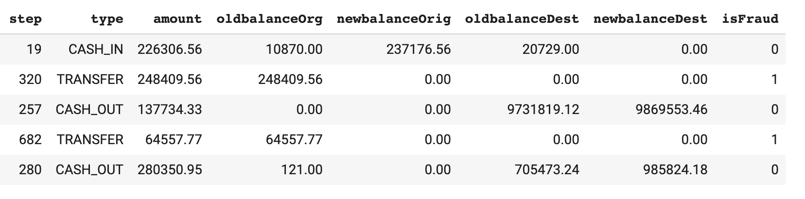
df = shuffle(df, random_state=2)

The resulting dataset contains 25% fraud cases with a total of ~40k rows. Much better. I’ve also removed the transaction ID fields from the original Kaggle dataset. Here’s a snapshot of the data we’ll be working with:

Building a boosted tree model with TensorFlow

Tree-based model have been shown to be effective for anomaly detection, which is what I’ll be using here. To my amazement, I only recently discovered that TensorFlow has a boosted tree classifier. There’s a great tutorial on it here, which is mostly what I followed to build the model.

Here are the numeric and categorical columns I’m using to build each tf.feature_column:

CATEGORICAL_COLUMNS = ['type']
NUMERIC_COLUMNS = ['step', 'amount', 'oldbalanceOrg', 'newbalanceOrig', 'oldbalanceDest', 'newbalanceDest']

You can see what the resulting feature columns look like in this gist. Next, it’s time to define our estimator. We can do this in one line of code:

model = tf.estimator.BoostedTreesClassifier(feature_columns,
                                          n_batches_per_layer=1)

And train it in another:

model.train(train_input_fn, max_steps=100)

When I ran the test set through this model, I got 99% accuracy. And don’t worry, I verified it was predicting the fraudulent cases correctly. It was 😉

Preparing the model for deployment

In order to deploy our model to Cloud AI Platform and make use of Explainable AI, we need to export it as a TensorFlow 1 SavedModel and save it in a Cloud Storage bucket.

We’ll export our model by defining the following serving input function:

def json_serving_input_fn():
  inputs = {}
  for feat in feature_columns:
      if feat.name == "type_indicator":
            inputs['type'] = tf.placeholder(shape=[None], name=feat.name, dtype=tf.string)
      else:
          inputs[feat.name] = tf.placeholder(shape=[None], name=feat.name, dtype=feat.dtype)
  return tf.estimator.export.ServingInputReceiver(inputs, inputs)

We can now export it directly to a Cloud Storage bucket:

export_path = est.export_saved_model(
    'gs://your/gcs/bucket',
    serving_input_receiver_fn=json_serving_input_fn
).decode('utf-8')

Next, we’ll use the handy saved_model_cli to inspect our model’s TensorFlow graph:

!saved_model_cli show --dir $export_path --all

I won’t paste the full output of that here, but it shows our model’s SignatureDef which is a fancy way of saying: the data our model expects when we serve it. In this case, we want separate explanations for each input to our model. This means that each input (transaction type, balance, etc.) should be a separate tensor in our SigDef. Here’s what the SigDef looks like for two inputs to our model:

inputs['step'] tensor_info:
    dtype: DT_FLOAT
    shape: (-1)
    name: step:0
inputs['type'] tensor_info:
    dtype: DT_STRING
    shape: (-1)
    name: type_indicator:0

We’ll need this info to tell the explainability service what it should explain.

Choosing a baseline for explainability

Explainability helps us answer the question:

“Why did our model think this was fraud?”

For tabular data, Cloud’s Explainable AI service works by returning attribution values for each feature. These values indicate how much a particular feature affected the prediction. Let’s say the amount of a particular transaction caused our model to increase its predicted fraud probability by 0.2%. You might be thinking “0.2% relative to what??”. That brings us to the cocncept of a baseline.

The baseline for our model is essentially what it’s comparing against. For models deployed on AI Platform, we can choose the baseline. We select the baseline value for each feature in our model, and the baseline prediction consequently becomes the value our model predicts when the features are set at the baseline.

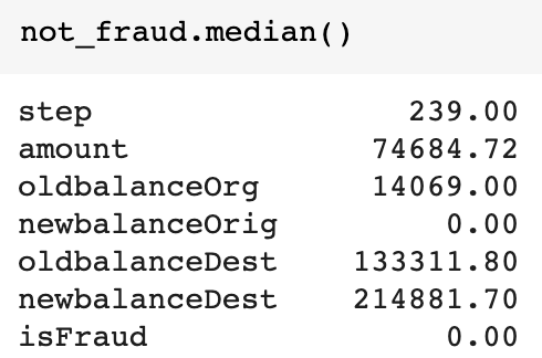
Choosing a baseline depends on the prediction task you’re solving. For numerical features, it’s common to use the median value of each feature in your dataset as the baseline. In the case of fraud detection, however, this isn’t exactly what we want. We care most about explaining the cases when our model labels a transaction as fraudulent. That means the baseline case we want to compare against is non-fraudulent transactions.

To account for this, we’ll use the median values of the non-fraudulent transactions in our dataset as the baseline. We can easily get the median in Pandas by calling not_fraud.median() on the DataFrame we created earlier containing only non-fraudulent transactions. Here’s the result:

For our categorical feature (transaction type), I chose the most frequently occurring value from our not fraud dataset. You can get this by running not_fraud['type'].value_counts(). In this case it’s CASH_OUT, which is what I used as the baseline for this feature.

When we deploy our explainable model to AI Platform, we tell the service our baselines by including them in an explanation_metadata.json file in the same GCS bucket as our SavedModel. I’ve put the code for creating the metadata file in this gist.

Each of our model’s features is an object in the inputs key, indicating the feature’s name in our model’s TensorFlow graph along with the baseline we should use for that feature:

"newbalanceDest": {
    "input_tensor_name": "newbalanceDest:0",
    "input_baselines": [not_fraud['newbalanceDest'].median()]
}

You’ll notice when we ran saved_model_cli above that we also got the name of our output tensor(s) in our model’s graph. We’ll need to include one of these in our explanation metadata file - it will tell the explanation service which output tensor to explain. For this example I’ve chosen the logistic tensor, which is a value ranging from 0 to 1 indicating the probability our model thinks each transaction is a fraud (1 being 100% confident something is a fraudulent transaction).

Deploying to Explainale AI

Now that all the pieces are in place, we can deploy our model to Cloud AI Platform with one gcloud command:

!gcloud beta ai-platform versions create $VERSION \
--model $MODEL \
--origin $export_path \
--runtime-version 1.15 \
--framework TENSORFLOW \
--python-version 3.5 \
--machine-type n1-standard-4 \
--explanation-method 'sampled-shapley' \
--num-paths 10

Notice that I’m using the Sampled Shapley explanation method, which supports explanations for non-differentiable models like this one (boosted tree models are not differentiable).

Getting predictions attribution values

If you made it this far, congrats! 👏👏👏

Time for my favorite part: model explanations. I’ve created a data.txt file with five fraudulent examples from my test set (remember, we only want to explain instances our model should label as fraud). Here’s what one line of that file looks like:

{"step": 679, "type": "TRANSFER", "amount": 403274.41, "oldbalanceOrg": 403274.41, "newbalanceOrig": 0.0, "oldbalanceDest": 0.0, "newbalanceDest": 0.0}

We’ll send that test data to our model for predictions and explanations using gcloud:

explanations = !gcloud beta ai-platform explain --model $MODEL --version $VERSION --json-instances='data.txt'
explain_dict = json.loads(explanations.s)

With that, you should have attribution values. I find them easier to understand visually so I’ve written some code to plot each example with matplotlib:

for i in explain_dict['explanations']:
    prediction_score = i['attributions_by_label'][0]['example_score']
    attributions = i['attributions_by_label'][0]['attributions']
    print('Model prediction:', prediction_score)
    fig, ax = plt.subplots()
    ax.barh(list(attributions.keys()), list(attributions.values()), align='center')
    plt.show()

We get this beautiful result:

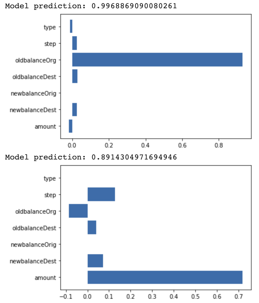
But what does it all mean? For the baseline values we chose above, our model’s baseline prediction is 0.019 or a 1.9% chance of fraud.

In the first example, the account’s initial balance before the transaction took place was the biggest indicator of fraud, pushing our model’s prediction up from the baseline more than 0.8.

In the second example, the amount of the transaction was the biggest indicator, followed by the step. In the dataset, the “step” represents a unit of time (1 step is 1 hour). Attribution values can also be negative. Our model was not quite as confident in this case (predicting 89% chance of fraud) due to the original balance feature.

What’s next?

As you’ve seen, lots can happen when you combine the power of TensorFlow boosted trees with explanations. Want to learn more? Check out these awesome resources:

• The AI Explainability whitepaper goes into a lot more detail on baselines and explanation methods
• For more on boosted tree models, this tutorial in the TF docs has you covered
• Dive into the docs on AI Platform explanations
• These notebooks show you how to deploy image and tabular models built with tf.keras to AI Platform explanations

As always, let me know what you thought of this post on Twitter at @SRobTweets.

Footnotes